Loading processed methylation data and checking beta distributions
Loading Beta Values and Metadata
We will continue working with the dataset referenced in the methylprep general walkthrough: GSE147391. It was processed from the command line with the following command:
>>> python -m methylprep process -d <filepath> --all
Where <filepath> is the directory where the raw IDAT files are stored. We use --all to tell methylprep to give us all the possible output files, which include:
- beta_values.pkl
- poobah_values.pkl
- control_probes.pkl
- m_values.pkl
- noob_meth_values.pkl
- noob_unmeth_values.pkl
- meth_values.pkl
- unmeth_values.pkl
- sample_sheet_meta_data.pkl
As well as folders that contain the processed methylation data in .csv files.
[1]:
import methylcheck
from pathlib import Path
filepath = Path('/Users/patriciagirardi/tutorial/GPL21145')

betas = methylcheck.load(filepath)
betas.head()
Files: 100%|██████████| 1/1 [00:00<00:00,  5.92it/s]
INFO:methylcheck.load_processed:loaded data (865859, 16) from 1 pickled files (0.222s)
[1]:
| 203163220027_R01C01 | 203163220027_R02C01 | 203163220027_R03C01 | 203163220027_R04C01 | 203163220027_R05C01 | 203163220027_R06C01 | 203163220027_R07C01 | 203163220027_R08C01 | 203175700025_R01C01 | 203175700025_R02C01 | 203175700025_R03C01 | 203175700025_R04C01 | 203175700025_R05C01 | 203175700025_R06C01 | 203175700025_R07C01 | 203175700025_R08C01 | |
|---|---|---|---|---|---|---|---|---|---|---|---|---|---|---|---|---|
| IlmnID | ||||||||||||||||
| cg00000029 | 0.852 | 0.749 | 0.739 | NaN | 0.891 | 0.896 | 0.757 | 0.734 | 0.806 | 0.881 | 0.740 | 0.885 | 0.693 | 0.779 | 0.617 | 0.891 |
| cg00000103 | NaN | NaN | NaN | NaN | NaN | NaN | NaN | NaN | NaN | NaN | NaN | NaN | NaN | NaN | NaN | NaN |
| cg00000109 | 0.943 | 0.916 | 0.884 | 0.951 | 0.936 | 0.774 | 0.932 | 0.920 | 0.898 | 0.938 | 0.931 | 0.953 | 0.899 | 0.889 | 0.734 | 0.892 |
| cg00000155 | 0.960 | 0.962 | 0.958 | 0.958 | 0.963 | 0.959 | 0.965 | 0.969 | 0.959 | 0.956 | 0.964 | 0.961 | 0.959 | 0.967 | 0.961 | 0.960 |
| cg00000158 | 0.969 | 0.972 | 0.971 | 0.968 | 0.968 | 0.964 | 0.970 | 0.974 | 0.964 | 0.969 | 0.960 | 0.968 | 0.965 | 0.965 | 0.975 | 0.966 |
You may also use methylcheck.load_both() to load both the beta values and metadata at the same time. Note that methylcheck expects the formatting used by methylprep in this command.
[2]:
df, meta = methylcheck.load_both(filepath)
meta.head()
INFO:methylcheck.load_processed:Found several meta_data files; attempting to match each with its respective beta_values files in same folders.
WARNING:methylcheck.load_processed:Columns in sample sheet meta data files does not match for these files and cannot be combined:['/Users/patriciagirardi/tutorial/GPL21145/GSE147391_GPL21145_meta_data.pkl', '/Users/patriciagirardi/tutorial/GPL21145/sample_sheet_meta_data.pkl']
INFO:methylcheck.load_processed:Multiple meta_data found. Only loading the first file.
INFO:methylcheck.load_processed:Loading 16 samples.
Files: 100%|██████████| 1/1 [00:00<00:00,  5.98it/s]
INFO:methylcheck.load_processed:loaded data (865859, 16) from 1 pickled files (0.2s)
INFO:methylcheck.load_processed:meta.Sample_IDs match data.index (OK)
[2]:
| GSM_ID | Sample_Name | Sentrix_ID | Sentrix_Position | source | histological diagnosis | description | Sample_ID | |
|---|---|---|---|---|---|---|---|---|
| 2 | GSM4429898 | Grade II rep3 | 203163220027 | R01C01 | Resected glioma | Diffuse astrocytoma (II) | Glioma | 203163220027_R01C01 |
| 3 | GSM4429899 | Grade III rep1 | 203163220027 | R02C01 | Resected glioma | Anaplastic astrocytoma (III) | Glioma | 203163220027_R02C01 |
| 12 | GSM4429908 | Grade IV rep5 | 203163220027 | R03C01 | Resected glioma | Glioblastoma (IV) | Glioma | 203163220027_R03C01 |
| 15 | GSM4429911 | Grade IV rep8 | 203163220027 | R04C01 | Resected glioma | Glioblastoma (IV) | Glioma | 203163220027_R04C01 |
| 6 | GSM4429902 | Grade II rep6 | 203163220027 | R05C01 | Resected glioma | Oligodendroglioma (II) | Glioma | 203163220027_R05C01 |
Loading Other Types of Data
Formats supported by methylcheck.load() are:
[‘beta_value’, ‘m_value’, ‘meth’, ‘meth_df’, ‘noob_df’, ‘sesame’, ‘beta_csv’]
where ‘beta_value’ is the default.
[3]:
# the unnormalized probe values
(meth,unmeth) = methylcheck.load(filepath, format='meth_df')
meth.head()
100%|██████████| 16/16 [00:00<00:00, 488.67it/s]
100%|██████████| 16/16 [00:00<00:00, 1480.91it/s]
INFO:methylcheck.load_processed:(865859, 16) (865859, 16)
[3]:
| 203163220027_R01C01 | 203163220027_R02C01 | 203163220027_R03C01 | 203163220027_R04C01 | 203163220027_R05C01 | 203163220027_R06C01 | 203163220027_R07C01 | 203163220027_R08C01 | 203175700025_R01C01 | 203175700025_R02C01 | 203175700025_R03C01 | 203175700025_R04C01 | 203175700025_R05C01 | 203175700025_R06C01 | 203175700025_R07C01 | 203175700025_R08C01 | |
|---|---|---|---|---|---|---|---|---|---|---|---|---|---|---|---|---|
| IlmnID | ||||||||||||||||
| cg00000029 | 933.0 | 874.0 | 845.0 | 528.0 | 1579.0 | 1243.0 | 893.0 | 741.0 | 1016.0 | 1272.0 | 1035.0 | 1423.0 | 917.0 | 904.0 | 743.0 | 1386.0 |
| cg00000103 | NaN | NaN | NaN | NaN | NaN | NaN | NaN | NaN | NaN | NaN | NaN | NaN | NaN | NaN | NaN | NaN |
| cg00000109 | 2597.0 | 2428.0 | 2309.0 | 3082.0 | 2542.0 | 2382.0 | 2710.0 | 1930.0 | 2029.0 | 2551.0 | 2385.0 | 3010.0 | 2219.0 | 1716.0 | 2132.0 | 2158.0 |
| cg00000155 | 3491.0 | 4397.0 | 3956.0 | 4059.0 | 4314.0 | 4059.0 | 4403.0 | 4302.0 | 3865.0 | 3734.0 | 4996.0 | 5297.0 | 3787.0 | 5216.0 | 4389.0 | 4404.0 |
| cg00000158 | 5556.0 | 5534.0 | 5384.0 | 4833.0 | 5381.0 | 6078.0 | 5678.0 | 4738.0 | 4938.0 | 4690.0 | 5658.0 | 6767.0 | 6030.0 | 5780.0 | 6300.0 | 5050.0 |
[4]:
# noob-normalized probe values
(noob_meth,noob_unmeth) = methylcheck.load(filepath, format='noob_df')
noob_meth.head()
100%|██████████| 16/16 [00:00<00:00, 550.34it/s]
100%|██████████| 16/16 [00:00<00:00, 1499.81it/s]
INFO:methylcheck.load_processed:(865859, 16), (865859, 16)
[4]:
| 203163220027_R01C01 | 203163220027_R02C01 | 203163220027_R03C01 | 203163220027_R04C01 | 203163220027_R05C01 | 203163220027_R06C01 | 203163220027_R07C01 | 203163220027_R08C01 | 203175700025_R01C01 | 203175700025_R02C01 | 203175700025_R03C01 | 203175700025_R04C01 | 203175700025_R05C01 | 203175700025_R06C01 | 203175700025_R07C01 | 203175700025_R08C01 | |
|---|---|---|---|---|---|---|---|---|---|---|---|---|---|---|---|---|
| IlmnID | ||||||||||||||||
| cg00000029 | 1174.0 | 1123.0 | 973.0 | NaN | 1745.0 | 1355.0 | 1074.0 | 812.0 | 1342.0 | 1497.0 | 1286.0 | 1696.0 | 1018.0 | 956.0 | 820.0 | 1524.0 |
| cg00000103 | NaN | NaN | NaN | NaN | NaN | NaN | NaN | NaN | NaN | NaN | NaN | NaN | NaN | NaN | NaN | NaN |
| cg00000109 | 3372.0 | 3003.0 | 2728.0 | 3645.0 | 2950.0 | 2766.0 | 3160.0 | 2185.0 | 2684.0 | 3191.0 | 2902.0 | 3526.0 | 2488.0 | 1883.0 | 2384.0 | 2368.0 |
| cg00000155 | 4647.0 | 5488.0 | 4754.0 | 4858.0 | 5390.0 | 5019.0 | 5198.0 | 5042.0 | 5300.0 | 4875.0 | 6244.0 | 6430.0 | 4254.0 | 6116.0 | 4892.0 | 5048.0 |
| cg00000158 | 7810.0 | 7100.0 | 6721.0 | 5904.0 | 6912.0 | 7875.0 | 6893.0 | 5625.0 | 6925.0 | 6278.0 | 7188.0 | 8478.0 | 7100.0 | 6859.0 | 7247.0 | 5887.0 |
[5]:
# m_values
m_values = methylcheck.load(filepath, format='m_value')
m_values.head()
Files: 100%|██████████| 1/1 [00:00<00:00,  5.41it/s]
INFO:methylcheck.load_processed:loaded data (865859, 16) from 1 pickled files (0.22s)
[5]:
| 203163220027_R01C01 | 203163220027_R02C01 | 203163220027_R03C01 | 203163220027_R04C01 | 203163220027_R05C01 | 203163220027_R06C01 | 203163220027_R07C01 | 203163220027_R08C01 | 203175700025_R01C01 | 203175700025_R02C01 | 203175700025_R03C01 | 203175700025_R04C01 | 203175700025_R05C01 | 203175700025_R06C01 | 203175700025_R07C01 | 203175700025_R08C01 | |
|---|---|---|---|---|---|---|---|---|---|---|---|---|---|---|---|---|
| IlmnID | ||||||||||||||||
| cg00000029 | 2.525 | 1.579 | 1.500 | NaN | 3.028 | 3.109 | 1.643 | 1.466 | 2.055 | 2.890 | 1.508 | 2.940 | 1.175 | 1.819 | 0.685 | 3.027 |
| cg00000103 | NaN | NaN | NaN | NaN | NaN | NaN | NaN | NaN | NaN | NaN | NaN | NaN | NaN | NaN | NaN | NaN |
| cg00000109 | 4.047 | 3.444 | 2.930 | 4.269 | 3.875 | 1.775 | 3.780 | 3.516 | 3.133 | 3.912 | 3.748 | 4.358 | 3.162 | 3.008 | 1.468 | 3.045 |
| cg00000155 | 4.582 | 4.681 | 4.528 | 4.518 | 4.717 | 4.538 | 4.797 | 4.960 | 4.564 | 4.444 | 4.738 | 4.606 | 4.547 | 4.885 | 4.641 | 4.567 |
| cg00000158 | 4.960 | 5.135 | 5.042 | 4.928 | 4.909 | 4.748 | 4.996 | 5.238 | 4.746 | 4.958 | 4.568 | 4.920 | 4.788 | 4.795 | 5.284 | 4.844 |
Note: If you point to a folder with multiple batches of samples, of different array types, you’ll get an error. All samples in the path you choose need to have the same number of probes (same array type). Here is the message you’ll get in this scenario.
ValueError: all the input array dimensions for the concatenation axis must match exactly,
but along dimension 0, the array at index 0 has size 226618 and the array at index 1 has size 244827
This shouldn’t happen if you download and process data using methylprep (which will automatically detect array types and create separate folders for each array type). If you didn’t process with methylprep, the workaround is manually moving the files from different array-types into separate folders and loading them separately.
The meth format for methylcheck.load() returns a list of SampleDataContainer objects.
sdc[0]._SampleDataContainer__data_frame will give you a dataframe of the first SampleDataContainer in your list called sdc.
Loading Data from .csv Files
methylcheck assumes you want to load data the fastest way, using a single high-performance python3 pickled dataframe. But there are times when you want to load from CSV output files instead. One use case is where you want to examine probes that were filtered out by poobah (p-value probe detection). The CSVs contain this information, whereas the pickled dataframe has it removed by default.
If you wish to load the beta values from CSVs, point the function to the parent directory where your CSVs are and it will automatically go through that directory recursively to concatinate all of the beta value columns from each CSV present. Please note that this will take longer than reading it from the beta pickle.
This function will by default mask the beta values of failed probes with NaN (p<=0.05). If you wish to view your raw beta values without any influence by poobah, add the argument no_poobah=True.
[6]:
df = methylcheck.load(filepath, format='beta_csv')
df
Files:   0%|          | 0/16 [00:00<?, ?it/s]INFO:numexpr.utils:NumExpr defaulting to 8 threads.
Files: 100%|██████████| 16/16 [00:20<00:00,  1.29s/it]
INFO:methylcheck.load_processed:merging...
100%|██████████| 16/16 [00:00<00:00, 524.09it/s]
[6]:
| 203163220027_R02C01 | 203163220027_R06C01 | 203163220027_R08C01 | 203163220027_R03C01 | 203163220027_R07C01 | 203163220027_R04C01 | 203163220027_R01C01 | 203163220027_R05C01 | 203175700025_R02C01 | 203175700025_R06C01 | 203175700025_R08C01 | 203175700025_R03C01 | 203175700025_R07C01 | 203175700025_R04C01 | 203175700025_R01C01 | 203175700025_R05C01 | |
|---|---|---|---|---|---|---|---|---|---|---|---|---|---|---|---|---|
| IlmnID | ||||||||||||||||
| cg00000029 | 0.749 | 0.896 | 0.734 | 0.739 | 0.757 | NaN | 0.852 | 0.891 | 0.881 | 0.779 | 0.891 | 0.740 | 0.617 | 0.885 | 0.806 | 0.693 |
| cg00000103 | 0.922 | 0.950 | 0.654 | 0.931 | 0.712 | 0.924 | 0.943 | 0.931 | 0.943 | 0.920 | 0.731 | 0.809 | 0.611 | 0.365 | 0.946 | 0.934 |
| cg00000109 | 0.916 | 0.774 | 0.920 | 0.884 | 0.932 | 0.951 | 0.943 | 0.936 | 0.938 | 0.889 | 0.892 | 0.931 | 0.734 | 0.953 | 0.898 | 0.899 |
| cg00000155 | 0.962 | 0.959 | 0.969 | 0.958 | 0.965 | 0.958 | 0.960 | 0.963 | 0.956 | 0.967 | 0.960 | 0.964 | 0.961 | 0.961 | 0.959 | 0.959 |
| cg00000158 | 0.972 | 0.964 | 0.974 | 0.971 | 0.970 | 0.968 | 0.969 | 0.968 | 0.969 | 0.965 | 0.966 | 0.960 | 0.975 | 0.968 | 0.964 | 0.965 |
| ... | ... | ... | ... | ... | ... | ... | ... | ... | ... | ... | ... | ... | ... | ... | ... | ... |
| rs9363764 | 0.544 | 0.544 | 0.592 | 0.062 | 0.058 | 0.431 | 0.962 | 0.036 | 0.046 | 0.562 | 0.046 | 0.054 | 0.541 | 0.551 | 0.971 | 0.966 |
| rs939290 | 0.055 | 0.591 | 0.974 | 0.051 | 0.965 | 0.809 | 0.966 | 0.070 | 0.964 | 0.578 | 0.601 | 0.535 | 0.625 | 0.603 | 0.962 | 0.965 |
| rs951295 | 0.557 | 0.032 | 0.566 | 0.515 | 0.955 | 0.966 | 0.548 | 0.975 | 0.024 | 0.073 | 0.556 | 0.035 | 0.974 | 0.523 | 0.029 | 0.949 |
| rs966367 | 0.966 | 0.468 | 0.028 | 0.956 | 0.499 | 0.036 | 0.029 | 0.478 | 0.488 | 0.483 | 0.526 | 0.034 | 0.455 | 0.034 | 0.027 | 0.051 |
| rs9839873 | 0.968 | 0.618 | 0.975 | 0.642 | 0.671 | 0.962 | 0.969 | 0.969 | 0.969 | 0.613 | 0.669 | 0.967 | 0.974 | 0.972 | 0.970 | 0.050 |
865918 rows × 16 columns
Checking Beta Distributions
One of the first steps users should take when loading their data is examining the beta distribution and ensuring that the expected bimodal distribution is present. Samples whose beta distributions don’t fit the bimodal distribution are more likely to be poor quality samples that need to be filtered out (you may be expecting a different distribution based on what kind of data you’re looking at, of course, but the standard is bimodal with peaks around 0 and 1).
methylcheck includes a beta density plot function that is similar to seaborn’s kde plot. If the sample size is small enough (<30), sample names will be included in the legend of the plot, so you may identify outlier samples easily.
[7]:
methylcheck.beta_density_plot(df)
WARNING:methylcheck.samples.postprocessQC:Your data contains 7585 missing probe values per sample, (121361 overall). For a list per sample, use verbose=True
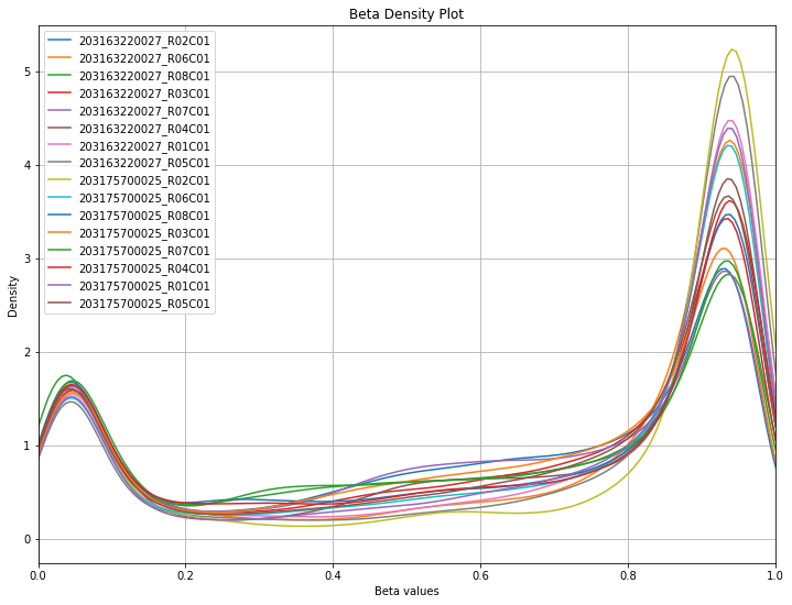
This data looks relatively clean! Most data on GEO should be high quality, but it always pays to check.
You may also want to get an idea of the mean beta distribution (useful for comparing multiple datasets, or for looking at a dataset before/after quality control measures.) Check the filtering probes section for examples on comparing beta distributions and what filtering can do to your data’s mean beta distribution.
[8]:
methylcheck.mean_beta_plot(df)
